Astrotools tutorial

This tutorial is meant to give a short overview about the different functionalities of the astrotools modules.

Module: coord.py

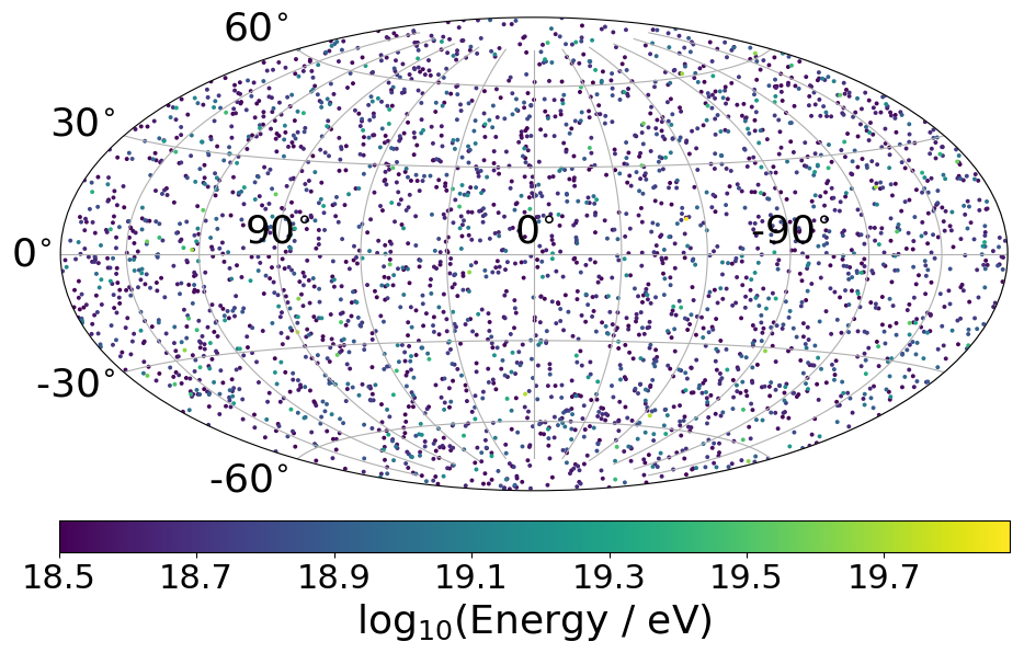
This modules converts between different coordinate systems. The following code snippet will show some basic setup of isotropic arrival directions in galactic coordinate system.

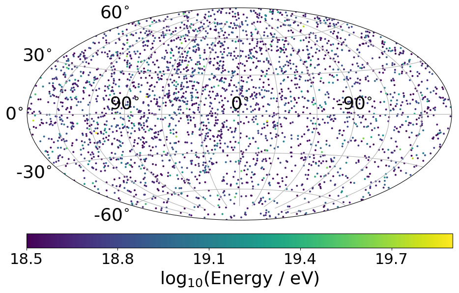
We create an isotropic arrival map and convert galactic longitudes (lons) and galactic latitudes (lats) into cartesian vectors.

from astrotools import auger, coord, skymap
ncrs, emin = 3000, 18.5            # number of cosmic rays
lons = coord.rand_phi(ncrs)        # isotropic in phi (~Uniform(-pi, pi))
lats = coord.rand_theta(ncrs)      # isotropic in theta (Uniform in cos(theta))
vecs = coord.ang2vec(lons, lats)   # or better directly: coord.rand_vec(ncrs)
# Plot an example map with sampled energies. If you specify the opath keyword in
# the skymap function, the plot will be automatically saved and closed
log10e = auger.rand_energy_from_auger(n=ncrs, log10e_min=emin)
skymap.scatter(vecs, c=log10e, opath='isotropic_sky.png')

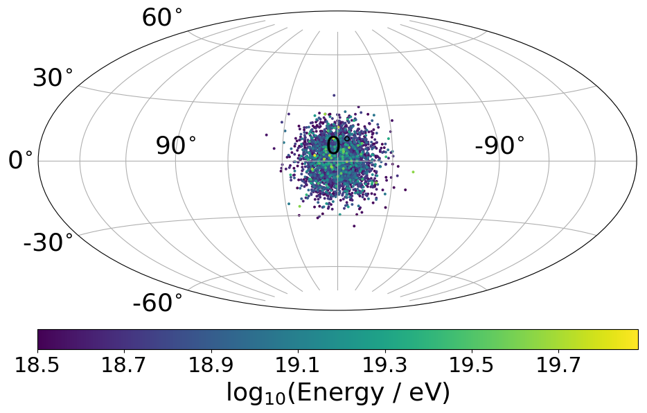
In the following code we create an arrival map with a source located at v_src=(1, 0, 0) and apply a fisher distribution around it with gaussian spread sigma=10 degree

import numpy as np
import matplotlib.pyplot as plt
v_src = np.array([1, 0, 0])
kappa = 1. / np.radians(10.)**2
vecs = coord.rand_fisher_vec(v_src, kappa=kappa, n=ncrs)
# if you dont specify the opath you can use (fig, ax) to plot more stuff
fig, ax = skymap.scatter(vecs, c=log10e)
plt.scatter(0, 0, s=100, c='red', marker='*')    # plot source in the center
plt.savefig('fisher_single_source_10deg.png', bbox_inches='tight')
plt.close()

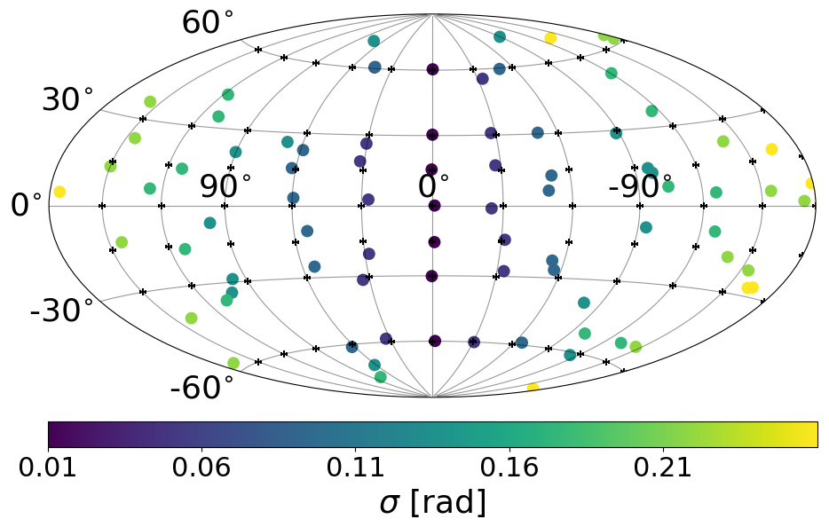
We can also use the coord.rand_fisher_vec() function to apply an angular uncertainty on simulated arrival directions by feeding a higher dimensional v_src in shape (3, ncrs). Each cosmic ray can also have a separate smearing angle, in the following code snippet increasing with the longitude.

lats = np.radians(np.array([-60, -30, -15, 0, 15, 30, 60]))
lons = np.radians(np.arange(-180, 180, 30))
lons, lats = np.meshgrid(lons, lats)
# vectors on this defined grid:
vecs = coord.ang2vec(lons.flatten(), lats.flatten())
# chose longitude dependent uncertainty
sigma = 0.01 + np.abs(lons.flatten()) / (4 * np.pi)
vecs_unc = coord.rand_fisher_vec(vecs, kappa=1/sigma**2)
skymap.scatter(vecs_unc, s=100, c=sigma, cblabel=r'$\sigma$ [rad]')
# To have the reference points we will also visualize the grid (Take care about the different longitude convention here)
plt.scatter(-lons.flatten(), lats.flatten(), marker='+', color='k')
plt.savefig('angular_uncertainty.png', bbox_inches='tight')
plt.close()

Module: healpytools.py

The healpytools provides an extension for the healpy framework (https://healpy.readthedocs.io), a tool to pixelize the sphere into cells with equal solid angle. There are various functionalities on top of healpy, e.g. sample random directions in pixel or create distributions on the sphere (dipole, fisher, experiment exposure).

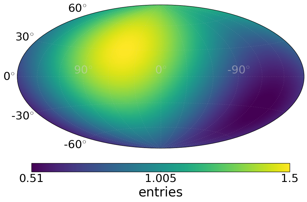
We will demonstrate some functions of the healpytools by creating a dipole distribution with amplitude 0.5 and direction of the maximum lon=45 degree and lat = 60 degree on the sphere. We first have to set the nside resolution parameter of healpy:

from astrotools import healpytools as hpt
nside = 64      # resolution of the HEALPix map (default: 64)
npix = hpt.nside2npix(nside)
nsets = 1000    # 1000 cosmic ray sets are created

lon, lat = np.radians(45), np.radians(60)   # Position of the maximum of the dipole (healpy and astrotools definition)
vec_max = hpt.ang2vec(lat, lon)             # Convert this to a vector
amplitude = 0.5                             # amplitude of dipole
dipole = hpt.dipole_pdf(nside, amplitude, vec_max, pdf=False)
skymap.heatmap(dipole, opath='dipole.png')

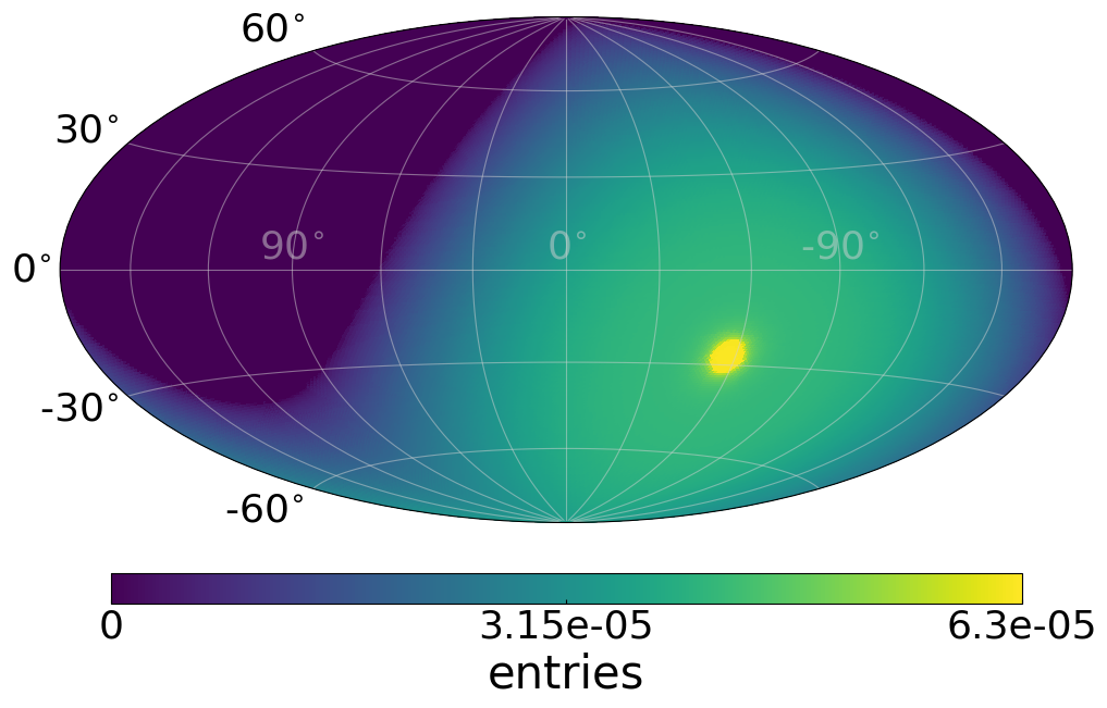
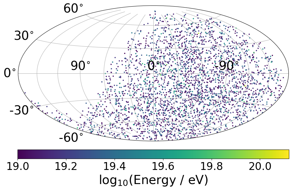
Now we want to sample 3000 cosmic ray events following this dipole distribution. As we are limited to the healpy resolution we will additionally sample random positions within each pixel cell:

pixel = hpt.rand_pix_from_map(dipole, n=3000)   # returns 3000 random pixel from this map
vecs = hpt.rand_vec_in_pix(nside, pixel)        # Random vectors within the drawn pixel
skymap.scatter(vecs, c=log10e, opath='dipole_events.png')

Create a healpy map that follows the exposure of an observatory at latitude a0 = -35.25 (Pierre Auger Observatory) and maximum zenith angle of 60 degree

exposure = hpt.exposure_pdf(nside, a0=-35.25, zmax=60)
skymap.heatmap(exposure, opath='exposure.png')

Note, if you want to sample from the exposure healpy map random vectors you have to be careful with the above method hpt.rand_vec_in_pix(), as the exposure healpy map reads out the exposure value in the pixel centers, whereas hpt.rand_vec_in_pix() might sample some directions where the exposure already dropped to zero. If you want to sample only isoptropic arrival directions it is instead recommended to use coord.rand_exposure_vec(), or if you can not avoid healpy pixelization use hpt.rand_exposure_vec_in_pix </code>.

Module cosmic_rays.py

This module provides a data container for cosmic ray observables and can be used to simply visualize, share, save and load data in an efficient way. There are two classes, the CosmicRaysBase and the CosmicRaysSets.

If you just have a single cosmic ray set you want to use the ComicRaysBase. You can set arbitrary content in the container. Objects with shape (self.crs) will be stored in an internal array called ‘shape_array’, all other data in a dictionary called ‘general_object_store’.

from astrotools import cosmic_rays
ncrs = 5000
lon, lat = hpt.pix2ang(nside, hpt.rand_pix_from_map(exposure, n=ncrs))
crs = cosmic_rays.CosmicRaysBase(ncrs)  # Initialize cosmic ray container
crs['lon'], crs['lat'] = lon, lat
crs['date'] = 'today'
crs['log10e'] = auger.rand_energy_from_auger(log10e_min=19, n=ncrs)
crs.set('vecs', coord.ang2vec(lon, lat))    # another possibility to set content
crs.keys()  # will print the keys that are existing

# Save, load and plot cosmic ray base container
opath = 'cr_base_container.npz'
crs.save(opath)
crs_load = cosmic_rays.CosmicRaysBase(opath)
crs_load.plot_heatmap(opath='cr_base_healpy.png')
crs_load.plot_eventmap(opath='cr_base_eventmap.png')

You can also quickly write all data in an usual ASCII file:

crs.save_readable('cr_base.txt')

For a big simulation with a lot of sets (simulated skys), you should use the CosmicRaysSets(). Inheriting from CosmicRaysBase(), objects with different shape than (nsets, ncrs) will be stored in the ‘general_object_store’ here.

nsets = 100
crs = cosmic_rays.CosmicRaysSets(nsets, ncrs)
crs['pixel'] = np.random.randint(0, npix, size=(crs.shape))
crs_set0 = crs[0]           # this indexing will return a CosmicRaysBase() object
crs_subset = crs[10:20]     # will return a subset as CosmicRaysSets() object

Module simulations.py

The simulation module is a tool to setup arrival simulations in a few lines of code. It is a wrapper for the core functions and is based on the data container provided by the cosmic_rays module. In the following we show a few examples how to quickly setup arrival maps.

nside = 64      # resolution of the HEALPix map (default: 64)
nsets = 1000    # 1000 cosmic ray sets are created

First we will create an isotropic map with AUGER energy spectrum above 10 EeV and no charges. AUGER’s exposure is applied.

plt.close("all")

from astrotools import simulations

sim = simulations.ObservedBound(nside, nsets, ncrs)    # Initialize the simulation with nsets cosmic ray sets and
                                                             # ncrs cosmic rays in each set
sim.set_energy(log10e_min=19.)                 # Set minimum energy of 10^(19.) eV (10 EeV), and AUGER energy spectrum
sim.apply_exposure()                           # Applying AUGER's exposure
sim.arrival_setup(fsig=0.)                     # 0% signal cosmic rays
crs = sim.get_data()                           # Getting the data (object of cosmic_rays.CosmicRaysSets())

crs.plot_eventmap(setid=0)                  # First map of cosmic ray sets is plotted.
plt.show()

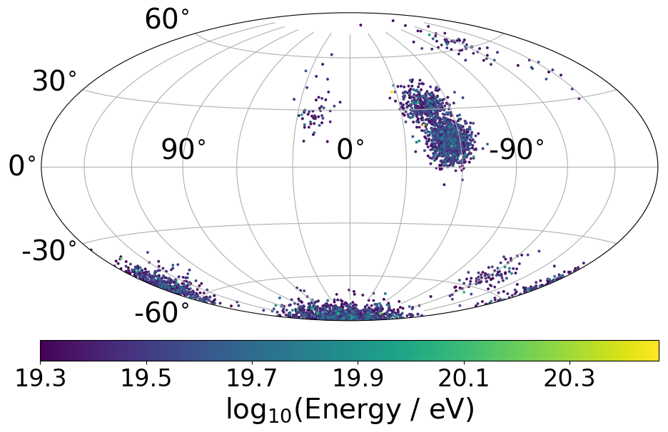
Now we create a 100% signal proton cosmic ray scenario (above 10^19.3 eV) from starburst galaxies with constant extragalactic smearing sigma=0.25. AUGER’s exposure is applied.

sim = simulations.ObservedBound(nside, nsets, ncrs)
sim.set_energy(log10e_min=19.3)             # Set minimum energy of 10^(19.3) eV, and AUGER energy spectrum (20 EeV)
sim.set_charges(charge=1.)                  # Set charge to Z=1 (proton)
sim.set_xmax('double')                      # Sample Xmax values from gumble distribution (assume A = 2*Z)
sim.set_sources(sources='sbg')              # Keyword for starburst galaxies. May also given an integer for number of
                                            # random placed sources or np.ndarray (x, y, z) of source positions.
sim.smear_sources(delta=0.1)                # constant smearing for fisher (kappa = 1/sigma^2)
sim.apply_exposure()                        # Applying AUGER's exposure
sim.arrival_setup(fsig=1.)                  # 100% signal cosmic rays
crs = sim.get_data()                        # Getting the data

crs.plot_eventmap(setid=0)                  # First map of cosmic ray sets is plotted.
plt.show()

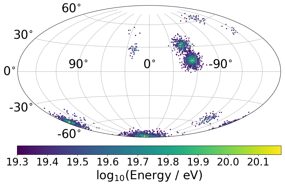
Finally, we create a 100% signal proton cosmic ray scenario (above 10^19.3 eV) from starburst galaxies with rigidity dependent extragalactic smearing (sigma = 0.1 / (10 * R[EV]) rad). AUGER’s exposure is applied and a signal fraction of 50 %.

sim = simulations.ObservedBound(nside, nsets, ncrs)
sim.set_energy(19.3)
sim.set_charges(1.)
sim.set_sources('sbg')
sim.set_rigidity_bins(np.arange(17., 20.48, 0.02) - 0.01)  # setting rigidity bins (either np.ndarray or the magnetic field lens)
sim.smear_sources(delta=0.2, dynamic=True)  # dynamic=True for rigidity dependent RMS deflection (sigma / R[10EV])
sim.apply_exposure()
sim.arrival_setup(fsig=0.5)
crs = sim.get_data()

crs.plot_eventmap(setid=0)
plt.show()

For usage of the galactic magnetic field lenses please refer to the test/tutorial/tutorial.py file in the repository.

Module gamale.py

The gamale (GAlactic MAgnetic LEns) module is a tool for handling galactic magnetic field lenses. The lenses can be created with the lens-factory: https://git.rwth-aachen.de/astro/lens-factory . Lenses provide information of the deflection of cosmic rays, consisting of matrices mapping a cosmic ray’s extragalactic origin to the observed direction on Earth. They are healpy based (https://healpy.readthedocs.io) and typically given in the nside=64 resolution to have an angular resolution of about 0.5 degrees. Thus, the matrices are of shape 49152 x 49152, and because of their size saved in scipy sparse format. Individual matrices (‘lens parts’) represent the deflection of particles in a specific rigidity range. One lens consists of multiple .npz-files (the lens parts) and a .cfg-file including information about the simulation and the rigidity range of the lens parts.

The following code requires a galactic field lens on your hard drive. First, we load the lens and a lens part.

# Loading a lens
lens_path = '/path/to/config/file.cfg'
lens = gamale.Lens(lens_path)

# Loading the lens part corresponding to a particle of energy log10e and charge z
log10e = 19  # Make sure that the rigidity is covered in your lens
z = 1
lens_part = lens.get_lens_part(loog10e=log10e, z=z)

# Alternatively, a lens part can be loaded directly
lens_part_path = '/path/to/lens/part.npz'
lens_part = gamale.load_lens_part(lens_part_path)

The lens part can be used to get the mapping between the extragalactic origin and the observed direction.

# Compute the observed directions of cosmic rays that arrives from direction of the
# extragalactic pixel eg_pix after backpropagation from earth. The amount of
# backpropagated cosmic rays per pixel is found as "Stat" in the .cfg-file.
eg_pix = np.random.randint(0, npix)
obs_dist = gamale.observed_vector(lens_part, eg_pix)  # Distribution of shape (Nside,)
print("A cosmic ray originating from pixel %i is most likely observed in pixel %i." % (eg_pix, np.argmax(obs_dist)))

# The other direction is also possible. Calculate the distribution of extragalactic
# directions for cosmic rays arriving in the observed direction 'obs_pix'.
obs_pix = np.random.randint(0, npix)
eg_dist = gamale.extragalactic_vector(lens_part, obs_pix)  # Distribution of shape (Nside,)
print("A cosmic ray observed in pixel %i most likely originated in pixel %i." % (obs_pix, np.argmax(eg_dist)))

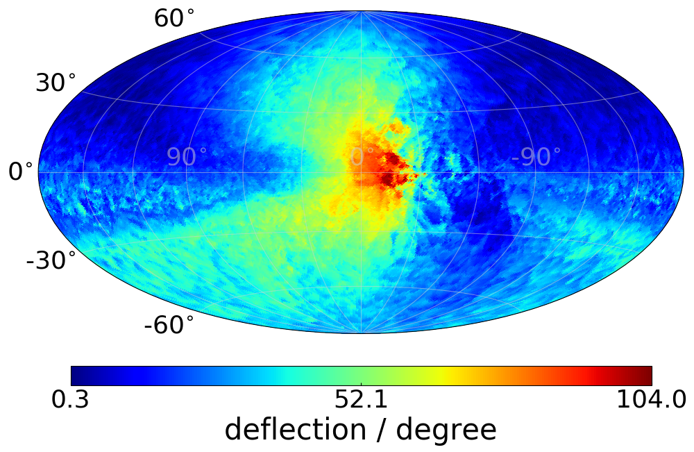
Gamale includes a function to automatically compute the mean deflection both for the complete lens part and direction dependent in form of a skymap.

# Calculating the mean deflection
mean_deflection = gamale.mean_deflection(lens_part)  # in radians
print("The mean deflection for this rigidity is %f degree." % np.rad2deg(mean_deflection))
# Mean deflection skymap
deflection_map = gamale.mean_deflection(lens_part, skymap=True)
skymap.heatmap(np.rad2deg(deflection_map), label='deflection / degree', cmap='jet', opath='deflection_map.png')

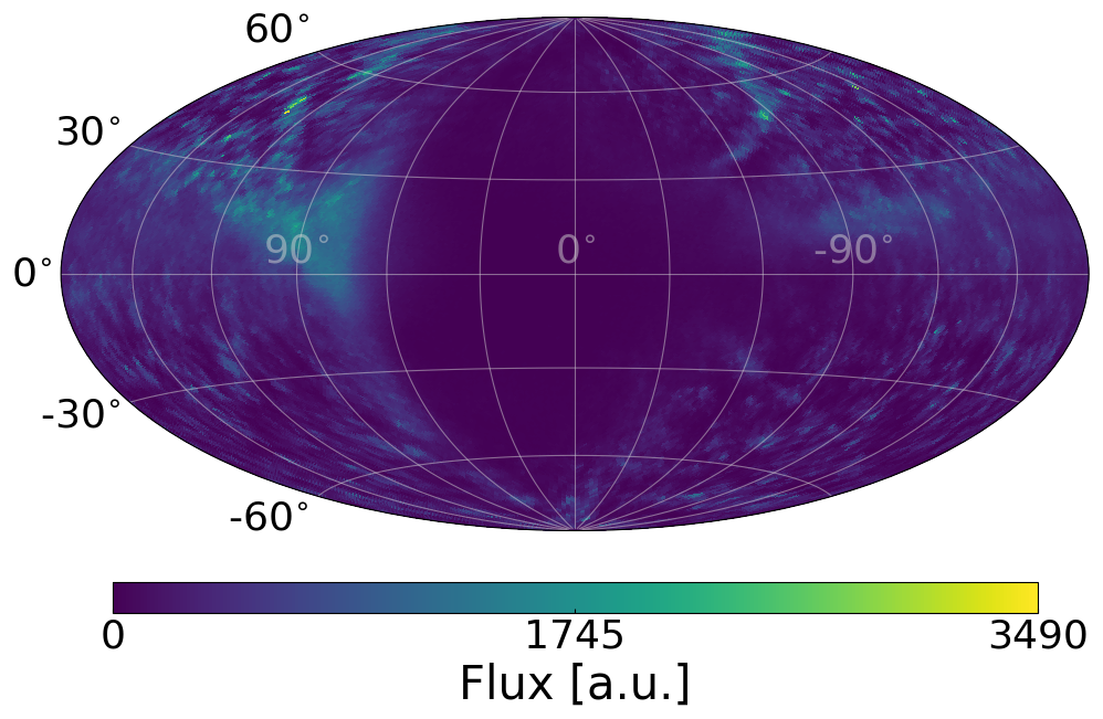
Using the observed_vector() function, it is possible to calculate the flux / transparency of the galactic magnetic field outside of the galaxy by computing the sum of all observed rays reaching Earth originating from the extragalactic pixel ‘pix’. The larger the amount of flux for that given pixel, the more likely a cosmic ray originating from that direction reaches Earth.

# brute force calculation of the flux map
flux = np.zeros(npix)
for pix in range(npix):
    flux[pix] = np.sum(gamale.observed_vector(lens_part, pix))

# gamale function to calculate the flux
flux = gamale.flux_map(lens_part)
skymap.heatmap(flux, label='Flux [a.u.]', opath='flux_map.png')

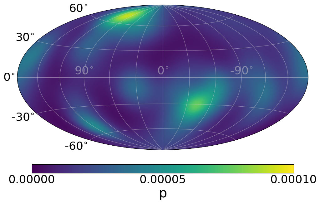
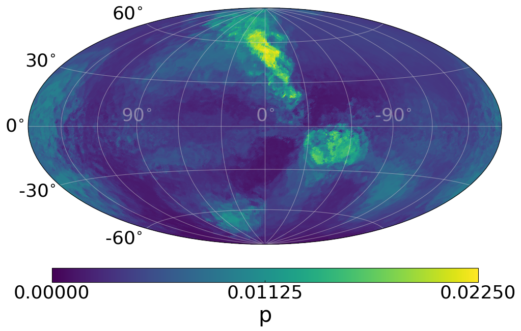
Finally, an entire probability distributions of extragalactic cosmic rays can be ‘lensed’ to Earth by a fast matrix multiplication:

# We create an extragalctic distributions of 30 gaussian source priors
eg_map = np.zeros(npix)
for i in range(30):
    v_src = coord.rand_vec()
    sigma = 10 + 10 * np.random.random()
    eg_map += hpt.fisher_pdf(nside, v_src, k=1/np.deg2rad(sigma)**2, sparse=False)
eg_map /= np.sum(eg_map)  # normalize to probability density distribution
skymap.heatmap(eg_map, label='p', opath='extragalactic_distribution.png')

# matrix multiplication to obtain an observed map
obs_map = lens_part.dot(eg_map)
skymap.heatmap(obs_map, label='p', opath='lensed_observed_distribution.png')

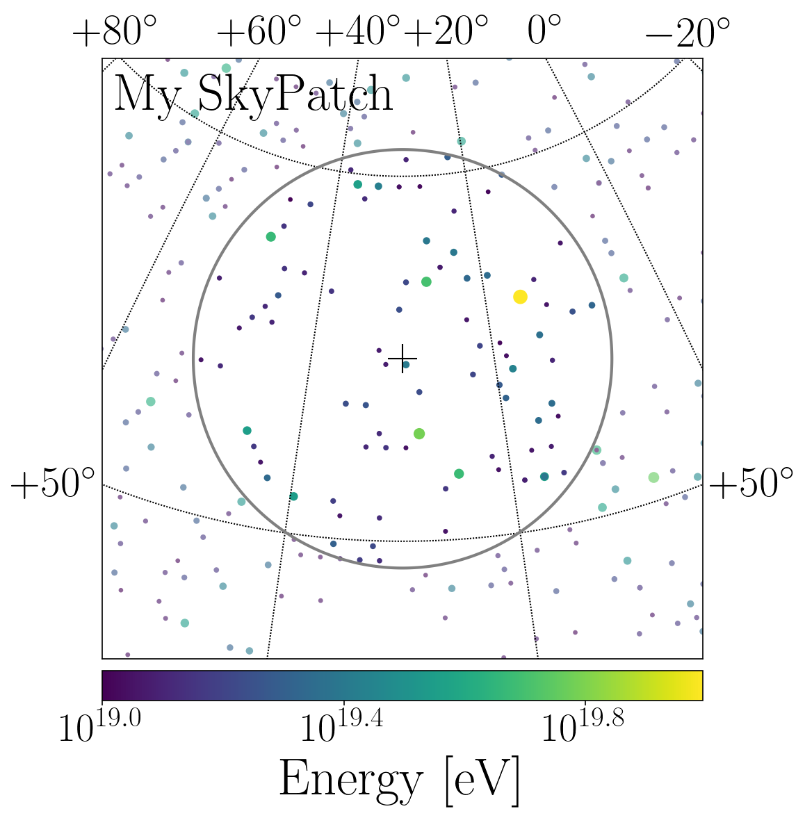
Module skymap.py

The skymap module have already been presented multiplet times in the tutorial so far. Still there is one special visualization of a close-up look, that is demonstrated in the following.

If you have installed the python package ‘basemap’ you can execute the following code:

# Assume we have an isotropic skymap
sim = simulations.ObservedBound(nside, nsets=2, ncrs=10000)
sim.set_energy(log10e_min=19.)                 # Set minimum energy of 10^(19.) eV (10 EeV), and AUGER energy spectrum
sim.arrival_setup(fsig=0.)                     # 0% signal cosmic rays
crs = sim.get_data()           # Getting the data (object of cosmic_rays.CosmicRaysSets())

Now we can setup a close-up view by specifying the coordinates of the region of interest (roi):

from astrotools.skymap import PlotSkyPatch
patch = PlotSkyPatch(lon_roi=np.deg2rad(30), lat_roi=np.deg2rad(60), r_roi=0.2, title='My SkyPatch')
mappable = patch.plot_crs(crs, set_idx=0)
patch.mark_roi()
patch.plot_grid()
patch.colorbar(mappable)
patch.savefig("skypatch.png")